(Encrypted) traffic mining
Introduction
Traffic Mining is the art of extracting hidden, obfuscated or encrypted information from IP traffic, by only observing the layer 2 to layer 4 header features. It exploits the fact that nobody produces perfect and secure code when writing Internet applications. The key points are libraries used by every one, such as audio codecs. They have intrinsic features and physical characteristics which cannot be changed without impeding correct functionality. This characteristic behavior reflects itself in layer 3 and 4 header features, independent of any encryption on layer 7. A prominent feature is the packet length (PL) and the inter-arrival time (IAT), also known as packet inter-distance, of the consecutive packets in an A or B flow.
Using these two parameters, not only the type of the traffic can be revealed, but also the content. To achieve this, two approaches of preprocessing are effective:
- Statistical approach (pktSIATHisto and descriptiveStats plugins)
- Signal processing approach (nFrstPkts plugin)
The major work in classification of encrypted traffic is the quality of the preprocessing. Hence, T2 focusses on what type of data should be fed into a classifier or a feature selection mechanism to produce optimal results.
In this tutorial, we will discuss these preprocessing approaches using the traffic from skypeu.pcap,
which contains a simple Skype voice conversation between two peers. For illustration t2plot, a wrapper for gnuplot is used.
Prerequisites
Create folders for your data and results
If you have not created a separate data and results directory yet, please do it now. This will greatly facilitate your workflow:
mkdir ~/data ~/results
Reset tranalyzer2 and the plugins configuration
If you have followed the other tutorials, you may have modified some of the core and plugins configuration. To ensure your results match those in this tutorial, make sure to reset everything:
t2conf -a --reset
You can also clean all build files:
t2build -a -c
Empty the plugin folder
To ensure we are not left with some unneeded plugins or plugins which were built using different core configuration, it is safer to empty the plugins folder:
t2build -e -y
Are you sure you want to empty the plugin folder '/home/user/.tranalyzer/plugins' (y/N)? yes
Plugin folder emptied
Download the PCAP files
The PCAP files used in this tutorial can be downloaded here:
Please save them in your ~/data folder:
wget --no-check-certificate -P ~/data https://tranalyzer.com/download/data/{film,skypeu}.pcap
Getting started
Build tranalyzer2 and the required plugins
For this tutorial, we will need to build the core (tranalyzer2) and the following plugins:
As you may have modified some of the automatically generated files, it is safer to use the -r and -f options.
...

BUILDING SUCCESSFUL
Run tranalyzer2
Now run t2 on skypeu.pcap:
t2 -r ~/data/skypeu.pcap -w ~/results
And look at the resulting files:
ls ~/results
skypeu_flows.txt skypeu_headers.txt
Troubleshooting
If you use your own pcap, which might contain flows with an abnormal, broad and diverse PL/IAT distribution,
t2 could terminate with the following message:
[ERR] pktSIATHisto: Failed to insert new tree node. Increase PSIAT_NDPLF in pktSIATHisto.h and recompile the plugin
Normally this should not happen, because the HISTO_NODEPOOL_FACTOR in pktSIATHisto.h is set to 17, which suffices for a large tree of PLs and IATs.
grep 'HISTO_NODEPOOL_FACTOR' $T2PLHOME/pktSIATHisto/src/pktSIATHisto.h
#define HISTO_NODEPOOL_FACTOR  17 // multiplication factor red-black tree nodepool:
                                  // sizeof(nodepool) = HISTO_NODEPOOL_FACTOR * mainHashMap->hashChainTableSize
Nevertheless, increase the HISTO_NODEPOOL_FACTOR to 18 or a bit higher:
t2conf pktSIATHisto -D HISTO_NODEPOOL_FACTOR=18
Recompile:
t2build pktSIATHisto
And see what happens when you re-run t2. If the message is accompanied by:
[WRN] Hash Autopilot: main HashMap full: flushing 1 oldest flow(s)!
[INF] Hash Autopilot: Fix: Invoke Tranalyzer with '-f value'
Then leave the HISTO_NODEPOOL_FACTOR alone and just restart t2 with the proposed -f value, e.g.,
t2 -r ~/data/your.pcap -w ~/results -f value
So now you are all set for any pcap mishap that might hit you in the future. Let’s start with the TM statistical approach.
Statistical approach
To profile traffic, the flow representation is the most convenient one, because the nature of a traffic type can be compressed into a collection of numbers, e.g., a vector, which can then be post-processed by standard programs such as Matlab, SPSS, Excel or by an AI plugin.
T2 produces several columns with statistical PL and IAT output. An excerpt is listed below from the header file: ~/results/skypeu_headers.txt
cat ~/results/skypeu_headers.txt
...
# Col No.   Type                        Name                        Description
...
23          U32                         nFpCnt                      Number of signal samples
24          U32_U64.U32:R               L2L3L4Pl_Iat                L2/L3/L4/Payload (s. PACKETLENGTH in packetCapture.h) length and IAT for the N first packets
25          U32                         tCnt                        Number of tree entries
26          U16_U32_U32_U32_U32:R       Ps_Iat_Cnt_PsCnt_IatCnt     Packet size (PS) and min inter-arrival time (IAT) of bin histogram
27          F                           dsMinPl                     Minimum packet length
28          F                           dsMaxPl                     Maximum packet length
29          F                           dsMeanPl                    Mean packet length
30          F                           dsLowQuartilePl             Lower quartile of packet lengths
31          F                           dsMedianPl                  Median of packet lengths
32          F                           dsUppQuartilePl             Upper quartile of packet lengths
33          F                           dsIqdPl                     Inter quartile distance of packet lengths
34          F                           dsModePl                    Mode of packet lengths
35          F                           dsRangePl                   Range of packet lengths
36          F                           dsStdPl                     Standard deviation of packet lengths
37          F                           dsRobStdPl                  Robust standard deviation of packet lengths
38          F                           dsSkewPl                    Skewness of packet lengths
39          F                           dsExcPl                     Excess of packet lengths
40          F                           dsMinIat                    Minimum inter arrival time
41          F                           dsMaxIat                    Maximum inter arrival time
42          F                           dsMeanIat                   Mean inter arrival time
43          F                           dsLowQuartileIat            Lower quartile of inter arrival times
44          F                           dsMedianIat                 Median inter arrival times
45          F                           dsUppQuartileIat            Upper quartile of inter arrival times
46          F                           dsIqdIat                    Inter quartile distance of inter arrival times
47          F                           dsModeIat                   Mode of inter arrival times
48          F                           dsRangeIat                  Range of inter arrival times
49          F                           dsStdIat                    Standard deviation of inter arrival times
50          F                           dsRobStdIat                 Robust standard deviation of inter arrival times
51          F                           dsSkewIat                   Skewness of inter arrival times
52          F                           dsExcIat                    Excess of inter arrival times
For now we are only interested in column 26 of ~/results/skypeu_flows.txt, namely Ps_Iat_Cnt_PsCnt_IatCnt. It contains a 3D statistics and their projections onto PL and IAT.
The packet length inter-arrival time distribution
An example of the PL/IAT distribution of pktSIATHisto for flowInd 1 is listed below
tawk 'flow(1) { print $dir, $Ps_Iat_Cnt_PsCnt_IatCnt }' ~/results/skypeu_flows.txt
%dir    Ps_Iat_Cnt_PsCnt_IatCnt
A       0_0_116_1078_213;0_1_7_1078_8;0_2_1_1078_1;0_7_1_1078_1;0_9_1_1078_2;0_10_2_1078_2;0_11_1_1078_1;0_12_2_1078_79;0_14_1_1078_1;0_25_1_1078_1;0_26_5_1078_5;0_27_3_1078_4;0_28_7_1078_8;0_29_4_1078_4;0_30_1_1078_1;0_31_1_1078_1;0_32_1_1078_3;0_39_5_1078_15;0_49_74_1078_120;0_50_134_1078_273;0_51_101_1078_342;0_52_167_1078_363;0_53_128_1078_208;...
B       0_0_89_1064_197;0_1_5_1064_5;0_3_1_1064_1;0_4_1_1064_1;0_5_2_1064_2;0_6_1_1064_1;0_7_1_1064_1;0_8_1_1064_1;0_9_3_1064_3;0_11_1_1064_5;0_20_1_1064_1;0_21_1_1064_2;0_23_1_1064_1;0_27_2_1064_3;0_28_3_1064_10;0_29_1_1064_1;0_32_1_1064_1;0_35_1_1064_1;0_39_11_1064_15;0_42_1_1064_1;0_44_1_1064_1;0_47_1_1064_1;0_49_14_1064_116;0_50_127_1064_235;...
Every scripting language, such as tawk, awk or perl have a split command which easily breaks up the line above and produces
arrays of elements to be further post-processed. Here is an example script:
tawk -H '{ n = split($Ps_Iat_Cnt_PsCnt_IatCnt, A, ";") for (i = 1; i <= n; i++) { split(A[i], B, "_") print B[2], B[1], B[3], B[4], B[5] } }’ ~/results/skypeu_flows.txt
0	0	116	1078	213
1	0	7	1078	8
2	0	1	1078	1
7	0	1	1078	1
9	0	1	1078	2
10	0	2	1078	2
11	0	1	1078	1
12	0	2	1078	79
14	0	1	1078	1
...
A more elaborate post-processing is provided by the script statGplt:
Generating '/home/user/results/skypeu_flows_ps.txt'... OK
Generating '/home/user/results/skypeu_flows_iat.txt'... OK
Generating '/home/user/results/skypeu_flows_ps_iat.txt'... OK
This will produce the following three files:
- skypeu_flows_ps.txt
- skypeu_flows_iat.txt
- skypeu_flows_ps_iat.txt
statGplt has a -P option to plot the packet length, IAT and the count as a 3D representation,
but for educational purposes, we will use the t2plot script instead:
t2plot -t "PL-IAT 3D statistics" -sy 0:100 -sx 0:40 -o 1:2:3 -v 60,45 ~/results/skypeu_flows_ps_iat.txt
This will result in the following graphics:
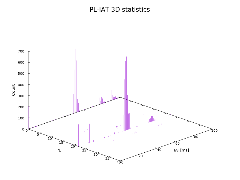
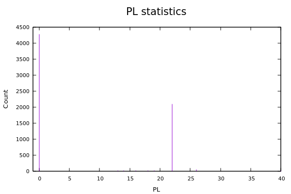
Or look at the projection, namely the packet length statistics. It contains information about the application.
t2plot -t "PL statistics" -sx -1:40 -o 1:2 ~/results/skypeu_flows_ps.txt
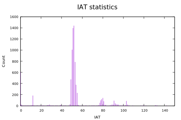
Sometimes the IAT statistics bears some information about the application and the user. But often the IAT alone is not significant enough.
t2plot -t "IAT statistics" -sx 0:150 -o 1:2 ~/results/skypeu_flows_iat.txt
Using the -r option, all online features of gnuplot can be used.
The PL/IAT, PL and IAT distributions can now be fed into a classifier of your choosing.
Now move to the packet size inter-arrival time plugin (pktSIATHisto):
pktSIATHisto
And look into the pktSIATHisto.h file.
vi src/pktSIATHisto.h
...
/* ========================================================================== */
/* ------------------------ USER CONFIGURATION FLAGS ------------------------ */
/* ========================================================================== */

#define PRINT_HISTO            1 // 1: print histo to flow file
#define HISTO_PRINT_BIN        0 // 1: Bin number; 0: Minimum of assigned inter arrival time.
                                 // (Example: Bin = 10 -> iat = [50:55) -> min(iat) = 50ms)

#define PSI_XCLD               0 // 1: include (PSI_XMIN, UINT16_MAX]
#define PSI_XMIN               1 // if (PSI_XCLD) minimal packet length starts at PSI_XMIN
#define PSI_MOD                0 // > 1: modulo factor of packet length

#define IATSECMAX              3 // max # of section in statistics, last section comprises all elements > IATBINBuN

//#define PSI_XMAX      UINT16_MAX // if (PSI_XCLD) maximal packet length

#define HISTO_EARLY_CLEANUP    0 // 1: after t2OnFlowTerminate tree information is destroyed
                                 // Do NOT switch on when dependent plugin, such as descriptiveStats is loaded!!
#define HISTO_DEBUG            0 // enables debug output

 // Bin boundary & width
#define IATBINBu1     200 // bin boundary of section one: [0, 200) ms
#define IATBINBu2     400
#define IATBINBu3    1000
#define IATBINBu4   10000
#define IATBINBu5  100000
#define IATBINBu6 1000000

#define IATBINWu1       1 // bin width 1ms
#define IATBINWu2       5
#define IATBINWu3      10
#define IATBINWu4      20
#define IATBINWu5      50
#define IATBINWu6     100

/* +++++++++++++++++++++ ENV / RUNTIME - conf Variables +++++++++++++++++++++ */

#define PSIAT_NDPLF    17 // multiplication factor red-black tree nodepool:
                          // sizeof(nodepool) = PSIAT_NDPLF * mainHashMap->hashChainTableSize

/* ========================================================================== */
/* ------------------------- DO NOT EDIT BELOW HERE ------------------------- */
/* ========================================================================== */
...
Change come into effect when the plugin is recompiled. To conserve flow memory space, the resolution of the IAT distribution can be flexibly configured to match the needs of the classifier. E.g., for voice applications the region between 0-400ms need to have a higher resolution than IAT > 1s. For other applications, it might be different. Hence, six sections are predefined, three are activated by setting IATSECMAX. The constant IATBINBu defines the upper boundary of a section while IATBINWu denotes the bin width. Thus, the resulting distribution can be expanded or shrunken to your linking. If more than 6 sections are necessary, you can add new defines and range definitions.
Nevertheless, especially for statistical classifiers or unsupervised learners, such as ESOM, a vector of constant dimensions is more appropriate. For that reason the descriptiveStats plugin was created, supplying PL and IAT statistics vectors up to the 3rd moment.
As the descriptiveStats plugin depends on the pktSIATHisto plugin the latter must ALWAYS be loaded as well.
Descriptive statistics
T2, or more precisely the descriptiveStats plugin, produces a descriptive statistics up to the 3rd moment from the PL/IAT distribution. Taking the pktSIATHisto data from ~/results/skypeu_flows.txt, for the A flow result in the following output:
tawk '(flow(1) && $dir == "A") || hdr() { print wildcard("^ds[A-Z]") }' ~/results/skypeu_flows.txt
dsMinPl  dsMaxPl  dsMeanPl  dsLowQuartilePl  dsMedianPl  dsUppQuartilePl  dsIqdPl  dsModePl  dsRangePl  dsStdPl   dsRobStdPl  dsSkewPl  dsExcPl   dsMinIat  dsMaxIat  dsMeanIat  dsLowQuartileIat  dsMedianIat  dsUppQuartileIat  dsIqdIat  dsModeIat  dsRangeIat  dsStdIat  dsRobStdIat  dsSkewIat  dsExcIat
0        967      11.79017  0                19          22               22       0         967        23.95365  16.3086     29.45955  1160.535  0.5       1000      53.04777   50.5              51.5         53.5              3         52.5       999.5       57.96778  2.2239       13.39272   213.7488
For each flow of a certain class, such a descriptive vector can be fed into a C5.0 or any other classifier for training and testing.
As our small example is not diverse enough, an example of ESOM clustering of unknown 2 GByte 1.7 Gbit/s traffic processed by T2 is depicted below. The resulting map arranges the unknown traffic type into regions, using only the PL descriptive vector.

The training of the map is derived by our own high performance post processing tool traviz3. Nevertheless, any AI tool can produce the same results. Maybe not with the same speed, but for research purposes they will do their job. Just import the PL vectors of your traffic of choice into Weka or Matlab.
Signal approach
The default configuration of the nFrstPkts plugin produces a signal of the first N packets per flow in ~/results/skypeu_flows.txt. In the default case, it will generate packet length (PL), inter-distance (IAT) tuples which is a well known feature in the traffic analysis community:
PL1_IAT1;PL2_IAT2;PL3_IAT3;...
tawk 'flow(1) { print $dir, $L2L3L4Pl_Iat }' ~/results/skypeu_flows.txt
%dir    L2L3L4Pl_Iat
A       0_0.000000;0_0.000140;14_0.021166;0_0.026188;107_0.000314;967_0.021067;0_0.051023;191_0.018234;0_0.061718;14_0.000392;0_5.527808;0_0.011243;0_0.051940;169_0.028764;...
B       0_0.000000;0_0.021295;14_0.026076;562_0.010252;485_0.022183;0_0.098612;70_0.021302;0_0.000507;22_5.486880;157_0.052041;80_0.051943;0_0.028936;22_0.000196;0_0.042731;...
A small tawk script easily breaks up the lines above and produces arrays of elements to be further post-processed, here is an example that produces a file
containing $L2L3L4Pl_Iat vectors from all flow indexes:
tawk -H '{ n = split($L2L3L4Pl_Iat, A, ";") for (i = 1; i <= n; i++) { split(A[i], B, "_") printf "%f%d", B[2], B[1] } }' ~/results/skypeu_flows.txt
0.000000	0
0.000140	0
0.021166	14
0.026188	0
0.000314	107
0.021067	967
0.051023	0
0.018234	191
...
An additional if can select certain flows of interest.
A more elaborate post-processing is provided by the script fpsGplt under tranalyzer2/scripts as an inspiration for you:
fpsGplt -h
Usage:
    fpsGplt [OPTION...] <FILE_flows.txt>

Optional arguments:
    -f findex        Flow index to extract [default: all flows]
    -d A|B           Flow direction: A or B only [default: A and B]

    -s               Time sorted ascending
    -t               No time, but counts on x axis [default: time on x axis]
    -i               Invert B flow PL
    -p s             Sample sorted signal with smplIAT in [s]; f = 1/smplIAT
    -e s             Time for each PL pulse edge in [s]

    -j               Calculate the jumps in IAT and report appropriate values
                     for MINIAT(S/U)

    -P               Plot the packet signal

    --gif  file      Generate a GIF file
    --jpeg file      Generate a JPEG file
    --png  file      Generate a PNG file
    --svg  file      Generate a SVG file

Help and documentation arguments:
    -h, --help       Show this help, then exit
The flow index, the flow direction and the time processing can be selected in order to produce the appropriate signal for your purpose. You will see its application later in this tutorial. Let us now discuss some prominent features of the plugin.
Signal preprocessing features nFrstPkts
In order to classify encrypted applications, normally the first 5-10 packets bear enough information because the initiation protocol reflects itself in these first PL/IAT sequences.
N depends on the type of job at hand.
For the first pcap supplied on the page, N=20 is enough.
For the second one, we will need a bigger value.
Nevertheless, you can select any N to your liking.
Just keep in mind that T2 has to hold all vectors times the amount of flows in memory.
So the performance of your machine is also a factor to consider.
The basic signal
The default configuration of nFrstPkts creates a standard PL/IAT vector per flow.
In order to produce a basic time based PL signal, the plugin needs to be configured.
The configuration options of the plugin can be found in the nFrstPkts.h file.
Let us move to the nFrstPkts directory using the nFrstPkts alias
nFrstPkts
and check the value of NFRST_IAT in the nFrstPkts.h file:
grep -Fw '#define NFRST_IAT' src/nFrstPkts.h
#define NFRST_IAT 1 // 0: Time relative to flow start; 1: Inter-arrival time; 2: Absolute timeAlternatively, we could have checked the current value of NFRST_IAT with t2conf -G:
t2conf nFrstPkts -G NFRST_IAT
NFRST_IAT = 1For this example, set NFRST_IAT to 0 by using t2conf
t2conf nFrstPkts -D NFRST_IAT=0
and then recompile the plugin:
t2build nFrstPkts
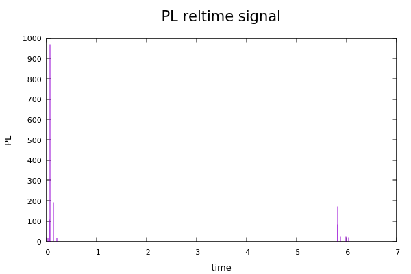
A packet length (PL) signal is produced, for each A/B flow starting at time = 0. This is convenient if time aligned vectors of each flow of a certain class is required e.g. to be presented to a neural net. So rerun T2
t2 -r ~/data/skypeu.pcap -w ~/results
The format of the nFrstPkts flow file output is listed below:
PL1_RelTime1;PL2_RelTime2;PL3_RelTime3;...
tawk 'flow(1) { print $dir, $L2L3L4Pl_Iat }' ~/results/skypeu_flows.txt
%dir    L2L3L4Pl_Iat
A       0_0.000000;0_0.000140;14_0.021306;0_0.047494;107_0.047808;967_0.068875;0_0.119898;191_0.138132;0_0.199850;14_0.200242;0_5.728050;0_5.739293;0_5.791233;169_5.819997;82_5.821208;22_5.872195;...
B       0_0.000000;0_0.021295;14_0.047371;562_0.057623;485_0.079806;0_0.178418;70_0.199720;0_0.200227;22_5.687107;157_5.739148;80_5.791091;0_5.820027;22_5.820223;0_5.862954;0_5.872205;22_5.927035;...
In order to produce file also readable by gnuplot and t2plot, run the fpsGplt script:
Generating '/home/wurst/results/skypeu_flows_nps.txt'... OK
cat ~/results/skypeu_flows_nps.txt
time        PL
0.000000    0
0.000140    0
0.021306    14
0.047494    0
0.047808    107
0.068875    967
0.119898    0
0.138132    191
0.199850    0
0.200242    14
5.728050    0
5.739293    0
5.791233    0
5.819997    169
5.821208    82
5.872195    22
5.968054    0
5.980476    22
6.032210    18
6.032504    0
And execute t2plot
t2plot -t "PL reltime signal" -o 1:2 -ws 600,400 ~/results/skypeu_flows_nps.txt
The signal processing approach treats the PLs of a flow as a digital signal. Due to the fact that packets do not appear at regular intervals, the resulting signal has missing samples (s. fig below).
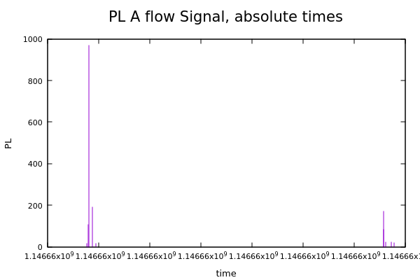
If NFRST_IAT is 2, then a signal vector is produced with absolute timestamps.
Let us use t2conf to change the value of NFRST_IAT, rebuild the plugin with t2build and
rerun t2:
t2conf nFrstPkts -D NFRST_IAT=2
t2build nFrstPkts
t2 -r ~/data/skypeu.pcap -w ~/results
The signal should now like that:
PL1_ATime1;PL2_ATime2;PL3_ATime3;...
tawk 'flow(1) { print $dir, $L2L3L4Pl_Iat }' ~/results/skypeu_flows.txt
%dir    L2L3L4Pl_Iat
A       0_1146661308.742778;0_1146661308.742918;14_1146661308.764084;0_1146661308.790272;107_1146661308.790586;967_1146661308.811653;0_1146661308.862676;191_1146661308.880910;0_1146661308.942628;14_1146661308.943020;0_1146661314.470828;...
B       0_1146661308.742876;0_1146661308.764171;14_1146661308.790247;562_1146661308.800499;485_1146661308.822682;0_1146661308.921294;70_1146661308.942596;0_1146661308.943103;22_1146661314.429983;157_1146661314.482024;80_1146661314.533967;...
We can now use the fpsGplt script to produce signal with A positive, B negative PL of flow index 1 and t2plot to display it:
Generating '/home/wurst/results/skypeu_flows_nps.txt'... OK
t2plot -t "PL symmetric A flow, absolute times" -o 1:2 -ws 600,400 ~/results/skypeu_flows_nps.txt
Signals are represented by complex numbers. They have amplitude and phase, a fact constantly ignored by some researchers. Nevertheless,
due to the nature of Internet traffic, sometimes a quick fix by omitting time makes classifiers more resilient. Hence, the script fpsGplt
has an additional parameter to replace time by an integer count, so a vector is produced by equidistant PL values, as depicted below.
Generating '/home/wurst/results/skypeu_flows_nps.txt'... OK
t2plot -t "PL signal" -o 1:2 -ws 600,400 ~/results/skypeu_flows_nps.txt
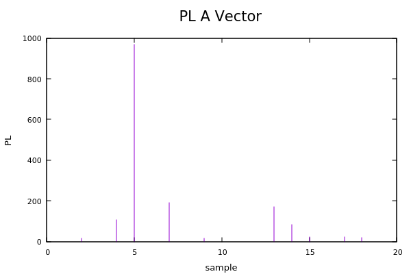
It is obvious that the spectrum of the signal is now drastically distorted, but the vector can be easily processed by any AI which requires abstract vectored input. Nevertheless, from the signal processing standpoint, this representation does not make so much sense, unless the number on the x-axis where correctly sampled values. So how do we get there without much computational effort?
One obvious approach is to pick the smallest IAT and use 2/IAT as a sampling frequency which often produces large vector dimensions and slows down the classification process.
Another approach is to reconstruct the signal with well known methods already used in radar technology. Here, a sampling frequency is picked outside a bandwidth limited signal according to Shannon’s requirements, which contains most of the energy of the original signal (Gerchberg Papadopulous). Been there, done that. Lots of computational effort, requires specialized HW if really being considered. But, then the missing samples can be reconstructed with a much lower frequency, producing less samples.
So a less expensive and easier way is required which almost satisfies dear old Shannon, and it has to be implemented in tranalyzer in a performant way. Satisfying Shannon is easy, he is dead, satisfying the Anteater is more difficult.
The A/B flow signal
The representation of a packet flow into a signal is vital. One method is to produce an A and B flow signal as depicted below. In order to preserve the causal correlation between A and B signals, the B part has to be shifted by the start of the B flow. We will see later that there are complications by just combining A and B flows into a signal, because the full duplex nature of the IP protocol and asymmetric delays of the peers do not guarantee causality between A and B packets. Leaving that aside, for the sake of simplicity, let’s first produce a signal which we can investigate and plot.
In this section, we will need to configure the NFRST_IAT and NFRST_BCORR flags. Let us quickly check their current value and documentation:
grep -Fw -e 'define NFRST_IAT' -e 'define NFRST_BCORR' $T2PLHOME/nFrstPkts/src/nFrstPkts.h
#define NFRST_IAT         2 // 0: Time relative to flow start; 1: Inter-arrival time; 2: Absolute time
#define NFRST_BCORR       0 // 0: A,B start at 0.0; 1: B shift by flow start; if (NFRST_IAT == 0)
Now, set NFRST_IAT to 0 and NFRST_BCORR to 1 with t2conf, then recompile the plugin and rerun t2:
t2conf nFrstPkts -D NFRST_IAT=0 -D NFRST_BCORR=1
t2build nFrstPkts
t2 -r ~/data/skypeu.pcap -w ~/results
If A and B flow are to be considered as one signal, then the B flow needs to be shifted by its start time. NFRST_BCORR set to 1 produces that operation, resulting in the following output
tawk 'flow(1) { print $dir, $L2L3L4Pl_Iat }' ~/results/skypeu_flows.txt
%dir    L2L3L4Pl_Iat
A       0_0.000000;0_0.000140;14_0.021306;0_0.047494;107_0.047808;967_0.068875;0_0.119898;191_0.138132;0_0.199850;14_0.200242;0_5.728050;0_5.739293;0_5.791233;169_5.819997;82_5.821208;22_5.872195;...
B       0_0.000098;0_0.021393;14_0.047469;562_0.057721;485_0.079904;0_0.178516;70_0.199818;0_0.200325;22_5.687205;157_5.739246;80_5.791189;0_5.820125;22_5.820321;0_5.863052;0_5.872303;22_5.927133;...
Note that the B signal starts at 0.000098, which is the start of the B flow.
A proper representation of the sequence above is the combined signal, where the B part is negated, thus also reducing the DC part in a natural way.
So use fpsGplt to extract flow 1 A/B part, B inverted (-i), calculate the jumps in IAT (-j) and invoke t2plot:
fpsGplt -h
Usage:
    fpsGplt [OPTION...] <FILE_flows.txt>

Optional arguments:
    -f findex        Flow index to extract [default: all flows]
    -d A|B           Flow direction: A or B only [default: A and B]

    -s               Time sorted ascending
    -t               No time, but counts on x axis [default: time on x axis]
    -i               Invert B flow PL
    -p s             Sample sorted signal with smplIAT in [s]; f = 1/smplIAT
    -e s             Time for each PL pulse edge in [s]

    -j               Calculate the jumps in IAT and report appropriate values
                     for MINIAT(S/U)

    -P               Plot the packet signal

    --gif  file      Generate a GIF file
    --jpeg file      Generate a JPEG file
    --png  file      Generate a PNG file
    --svg  file      Generate a SVG file

Help and documentation arguments:
-h, --help Show this help, then exitGenerating '/home/wurst/results/skypeu_flows_nps.txt'... OK Generating '/home/wurst/results/skypeu_flows_iat_jmp.txt'... OK
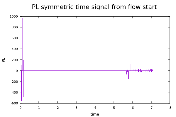
t2plot -t "PL symmetric time signal from flow start" -o 1:2 -ws 600,400 ~/results/skypeu_flows_nps.txt
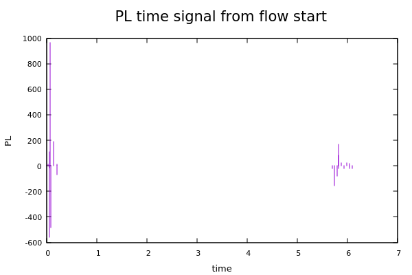
Zooming into the first part of the signal (right mouse click defines the area), we see a small B spike followed by a
larger A peak. Alternatively, rerun t2plot using the -sx option to specify the x range to display:
t2plot -t "PL symmetric time signal from flow start" -o 1:2 -ws 600,400 ~/results/skypeu_flows_nps.txt -sx 0.043:0.071
The smallest difference between A and B peak normally defines the minimum sampling frequency, which we like to be as low as possible
to reduce the amount of unnecessary sampled 0 and for performance reasons. Let’s see what happens if we omit this A-B packet
minimal inter-distance information and treat each flow separately to produce a signal which can be readily sampled with
a lower enough frequency. Have a look at the PL/IAT vector above and pick the minimum required pulse length for your sampling frequency. (awkf is just an alias for awk -F'\t' -v OFS='\t')
0.000000
0.000097
0.000139
0.000140
0.000191
0.000196
0.000281
0.000294
0.000314
0.000334
0.000392
0.000397
0.000507
0.000525
0.001196
0.001211
0.009251  <----- 1. large jump in reltime
0.009259
0.010159
0.010252
0.011235
...
Looking also at the plot above you will notice the bursty nature of the packet length signal. The task is to replace the spikes with an appropriate pulse length allowing a minimal sampling frequency. Looking at the sorted IAT list above, a drastic jump at 0.009251 can be identified. Thus any aggregation IAT below 9000us would be fine. Lets choose 2000us because 1ms is a reasonable unit for voice traffic. The minimal default pulse width is defined by NFRST_MINIAT(S/U)/NFRST_MINPLENFRC in nFrstPkts.h. The default value of NFRST_MINPLENFRC is 2.
The -j option of fpsGplt helps you to make the decision about the best MINIAT(S/U):
NFRST_MINIATS: 0, NFRST_MINIATU: 97, diff: 0.000097
NFRST_MINIATS: 0, NFRST_MINIATU: 294, diff: 0.000098
NFRST_MINIATS: 0, NFRST_MINIATU: 506, diff: 0.000115
NFRST_MINIATS: 0, NFRST_MINIATU: 1211, diff: 0.000704
NFRST_MINIATS: 0, NFRST_MINIATU: 9251, diff: 0.008040   <---- 1. large jump in IAT difference
NFRST_MINIATS: 0, NFRST_MINIATU: 42731, diff: 0.013795
NFRST_MINIATS: 0, NFRST_MINIATU: 95859, diff: 0.034141
NFRST_MINIATS: 5, NFRST_MINIATU: 486880, diff: 5.388268
Construction of a scannable signal
An obvious advantage of this aggregated flow signal representation in nFrstPkts is also the reduction of flow storage, as samples with packet length 0 are not needed anymore for signal by any post processing. This behavior is controlled by the NFRST_MINIATS and NFRST_MINIATU configuration flags:
grep -Fw -e '#define NFRST_MINIATS' -e '#define NFRST_MINIATU' $T2PLHOME/nFrstPkts/src/nFrstPkts.h
#define NFRST_MINIATS     0 // minimal IAT sec to define a pulse
#define NFRST_MINIATU     0 // minimal IAT usec to define a pulse
Let us set NFRST_MINIATU to 2000 with t2conf, recompile the plugin, rerun t2 and extract the flow 1 (A/B part) with fpsGplt.
t2conf nFrstPkts -D NFRST_MINIATU=2000
t2build nFrstPkts
t2 -r ~/data/skypeu.pcap -w ~/results
fpsGplt -f 1 -i ~/results/skypeu_flows.txt
Generating '/home/wurst/results/skypeu_flows_nps.txt'... OK
The format is then as follows: PL1_ReltimeSpike_PulseLength;PL2_ReltimeSpike_PulseLength;PL3_ReltimeSpike_PulseLength;...
tawk 'flow(1) { print $dir, $L2L3L4Pl_Iat_nP }' ~/results/skypeu_flows.txt
%dir L2L3L4Pl_Iat
A 14_0.021306_0.001000;107_0.047808_0.001000;967_0.068875_0.001000;191_0.138132_0.001000;14_0.200242_0.001000;125_5.819997_0.002211;22_5.872195_0.001000;22_5.980476_0.001000;18_6.032210_0.001000;22_6.084144_0.001000;22_6.192150_0.001000;...
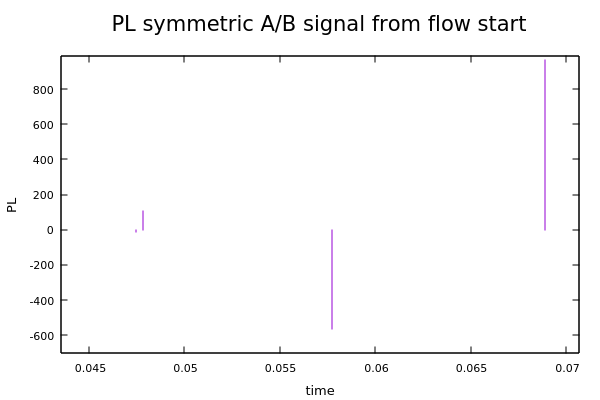
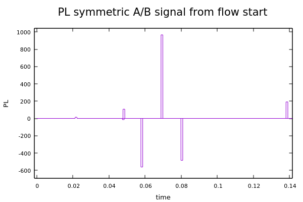
B 14_0.047469_0.001000;562_0.057721_0.001000;485_0.079904_0.001000;70_0.199818_0.001000;22_5.687205_0.001000;157_5.739246_0.001000;80_5.791189_0.001000;22_5.820321_0.001000;22_5.927133_0.001000;22_6.032473_0.001000;18_6.084457_0.001000;...Now invoke t2plot using the -pl option, so that PL values are connected. This facilitates the recognition of signal characteristics.
t2plot -t "PL symmetric A/B signal from flow start" -o 1:2 -pl -ws 600,400 ~/results/skypeu_flows_nps.txt
By using the -r option, you can use all mouse driven actions and look in detail at the signal by zooming using your mouse (ctrl wheel up).
For more gnuplot mouse commands type
gnuplot
show bind... <wheel-up> scroll up (in +Y direction) <wheel-down> scroll down <shift-wheel-up> scroll left (in -X direction) <shift-wheel-down> scroll right <Control-WheelUp> zoom in on mouse position <Control-WheelDown> zoom out on mouse position ...
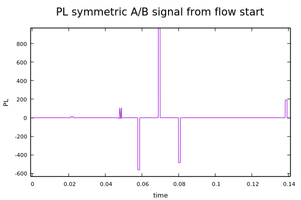
Alternatively, use t2plot -sx to specify the range to display:
t2plot -t "PL symmetric A/B signal from flow start absolute times, zoom" -o 1:2 -pl -ws 600,400 /home/wurst/results/skypeu_flows_nps_srt.txt -sx 0:0.142
<figure>
<a href="#" data-featherlight="/assets/img/LsigABShftSrtzm.png">
<img class="img" style="max-width: 100%" src="/assets/img/LsigABShftSrtzm.png">
</a>
<figcaption>Packet Length Signal: flowInd 1, A/B flow, reltime, B shifted, zoom</figcaption>
</figure>
<!---->
Note that around 0.044s, an A pulse is overlapping the B pulse. That is the effect mentioned before that IAT between A and B packets
are not considered to avoid high sampling frequencies. Sure enough, this is what needs to be done if we are really interested in being thorough.
An easy way to mitigate this effect is to consider A and B flow separately.
One approach is to shift every conflicting B pulse to the future, which tampers with the phase of the signal. For classification
purposes, a pragmatic choice. For signal freaks, a no-go. They will get the minimum A/B spike IAT and use a fraction of that as
a pulse length.
Because the A/B vectors are stored in sequence, the `-pl` option of `t2plot` plots lines crossing the pulse at 0. To produce a
consistent signal sorting by time is required.
<kbd>
awkf \'NR != 1\' ~/results/skypeu_flows_nps.txt | LC_ALL=C sort -t$\'\t\' -k1,1 | awkf \'BEGIN { print \"time\", \"PL\" } { print }\' > ~/results/skypeu_flows_nps_srt.txt
</kbd>
This works as well:
<kbd>
fpsGplt -f 1 -i -s ~/results/skypeu_flows.txt
</kbd>
<pre><samp>
Generating '/home/wurst/results/skypeu_flows_nps.txt'... <span class="code-ok">OK</span>
Generating '/home/wurst/results/skypeu_flows_nps_srt.txt'... <span class="code-ok">OK</span>
</samp></pre>
<kbd>
t2plot -t \"PL symmetric A/B signal from flow start absolute times, zoom\" -o 1:2 -pl -sx 0:0.142 -ws 600,400 ~/results/skypeu_flows_nps_srt.txt
</kbd>
<figure>
<a href="#" data-featherlight="/assets/img/LsigABShftSrtAzmS.png">
<img class="img" style="max-width: 100%" src="/assets/img/LsigABShftSrtAzmS.png">
</a>
<figcaption>Packet Length Signal: flowInd 1, A/B flow, reltime, B shifted, average PL, zoom</figcaption>
</figure>
<!---->
The peaky signal around 0.044s is the overlapping A/B signal effect described above.
To conclude this tutorial, let's configure *nFrsPkts.h* as follows for the next pcap:
```c
...
/* ========================================================================== */
/* ------------------------ USER CONFIGURATION FLAGS ------------------------ */
/* ========================================================================== */
#define NFRST_IAT 0 // 0: Time relative to flow start;
// 1: Inter-arrival time;
// 2: Absolute time
#define NFRST_BCORR 1 // 0: A,B start at 0.0;
// 1: B shift by flow start; if (NFRST_IAT == 0)
#define NFRST_MINIATS 0 // Minimal IAT sec to define a pulse
#define NFRST_MINIATU 0 // Minimal IAT usec to define a pulse
#define NFRST_MINPLENFRC 2 // Minimal pulse length fraction
#define NFRST_PLAVE 1 // 1: Packet Length Average;
// 0: Sum(PL) (BPP); if (NFRST_MINIATS|NFRST_MINIATU) > 0
#define NFRST_PKTCNT 200 // Define how many first packets are recorded
#define NFRST_HDRINFO 0 // Add L3 and L4 header length
#define NFRST_XCLD 0 // 0: include all,
// 1: include [NFRST_XMIN,NFRST_XMAX]
#define NFRST_XMIN 1 // Min PL boundary; NFRST_XCLD=1
#define NFRST_XMAX UINT16_MAX // Max PL boundary; NFRST_XCLD=1
/* ========================================================================== */
/* ------------------------- DO NOT EDIT BELOW HERE ------------------------- */
/* ========================================================================== */
...This can be achieved with t2conf as follows:
t2conf nFrstPkts -D NFRST_IAT=0 -D NFRST_BCORR=1 -D NFRST_MINIATS=0 -D NFRST_MINIATU=0 -D NFRST_MINPLENFRC=2 -D NFRST_PLAVE=1 -D NFRST_PKTCNT=200 -D NFRST_HDRINFO=0 -D NFRST_XCLD=0 -D NFRST_XMIN=1 -D NFRST_XMAX=UINT16_MAX
You can add the L3/4 header length to the PL by setting NFRST_HDRINFO. But then, all discussed signal forming modes will be deactivated. The NFRST_XCLD controls the exclusion of a certain PL range. The range is defined by NFRST_XMIN, NFRST_XMAX This is useful when certain PLs are not relevant for the classification process. Instead of weeding them out by the classifier itself, we can remove them before, thus reducing the size of the model or facilitating the feature extraction process.
Analyzing traffic of a film being streamed
Now download a more complicated PCAP where somebody streams a film: film.pcap
t2build nFrstPkts
t2 -r ~/data/film.pcap -w ~/results
fpsGplt -f 13 -i -s ~/results/film_flows.txtGenerating '/home/wurst/results/film_flows_nps.txt'... OK Generating '/home/wurst/results/film_flows_nps_srt.txt'... OK
t2plot -t "PL symmetric A/B signal from flow start" -o 1:2 -ws 600,400 ~/results/film_flows_nps_srt.txt
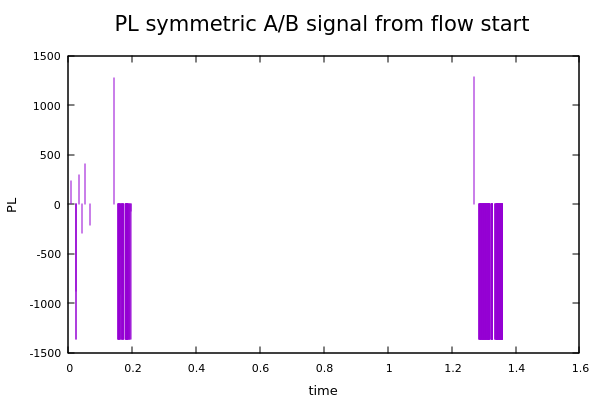
In order to produce a signal which can be used in AI applications or as a valid sample signal, minimal pulse length has
to be estimated. So set the NFRST_IAT parameter to 1, recompile the plugin, execute T2 and run fpsGplt for the whole flow with the -j option:
t2conf nFrstPkts -D NFRST_IAT=1
t2build nFrstPkts
t2 -r ~/data/film.pcap -w ~/results
fpsGplt -f 13 -j ~/results/film_flows.txtGenerating '/home/wurst/results/film_flows_nps.txt'... OK Generating '/home/wurst/results/film_flows_iat_jmp.txt'... OKcat ~/results/film_flows_iat_jmp.txt
NFRST_MINIATS: 0, NFRST_MINIATU: 1, diff: 0.000001 NFRST_MINIATS: 0, NFRST_MINIATU: 3, diff: 0.000001 NFRST_MINIATS: 0, NFRST_MINIATU: 5, diff: 0.000001 NFRST_MINIATS: 0, NFRST_MINIATU: 34, diff: 0.000029 NFRST_MINIATS: 0, NFRST_MINIATU: 195, diff: 0.000075 NFRST_MINIATS: 0, NFRST_MINIATU: 1596, diff: 0.000086 <--- 1. try 500-1500 NFRST_MINIATS: 0, NFRST_MINIATU: 1849, diff: 0.000107 NFRST_MINIATS: 0, NFRST_MINIATU: 2752, diff: 0.000199 <--- 2. try 2000 NFRST_MINIATS: 0, NFRST_MINIATU: 3075, diff: 0.000285 NFRST_MINIATS: 0, NFRST_MINIATU: 3724, diff: 0.000521 NFRST_MINIATS: 0, NFRST_MINIATU: 5582, diff: 0.000580 <--- 3. try 4000 NFRST_MINIATS: 0, NFRST_MINIATU: 9400, diff: 0.003818 <--- 4. try 6000 - 9000 NFRST_MINIATS: 0, NFRST_MINIATU: 72384, diff: 0.049071 <--- 5. try 20000 - 60000 NFRST_MINIATS: 1, NFRST_MINIATU: 73796, diff: 0.985782
So let’s try 2000 for a start and set NFRST_IAT to relative mode, i.e., 0.
Again rebuild the plugin, rerun t2 and fpsGplt, then plot the result with t2plot:
t2conf nFrstPkts -D NFRST_IAT=0 -D NFRST_MINIATS=0 -D NFRST_MINIATU=2000
t2build nFrstPkts
t2 -r ~/data/film.pcap -w ~/results
fpsGplt -f 13 -i -s ~/results/film_flows.txtGenerating '/home/wurst/results/film_flows_nps.txt'... OK Generating '/home/wurst/results/film_flows_nps_srt.txt'... OK
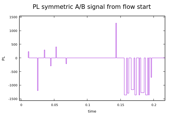
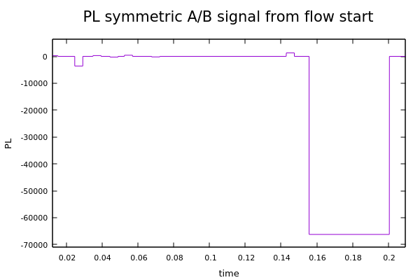
t2plot -t "PL symmetric A/B signal from flow start" -o 1:2 -pl -sx 0:0.22 -ws 600,400 ~/results/film_flows_nps_srt.txt
Now, let’s try with the 4th value:
t2conf nFrstPkts -D NFRST_MINIATU=9000
t2build nFrstPkts
t2 -r ~/data/film.pcap -w ~/results
fpsGplt -f 13 -i -s ~/results/film_flows.txtGenerating '/home/wurst/results/film_flows_nps.txt'... OK Generating '/home/wurst/results/film_flows_nps_srt.txt'... OK
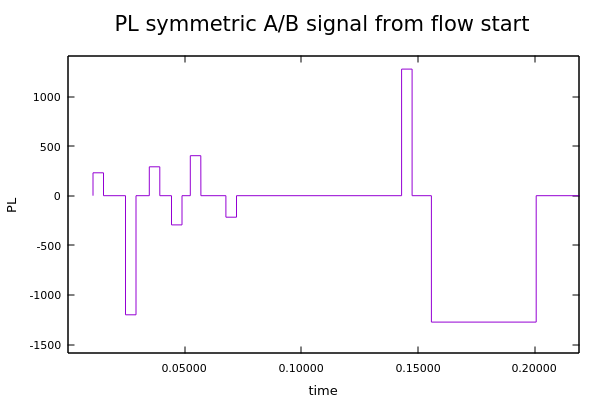
t2plot -t "PL symmetric A/B signal from flow start, zoom" -o 1:2 -pl -sx 0:0.22 -ws 600,400 ~/results/film_flows_nps_srt.txt
The edge of the pulses is controllable via the -e option. The default edge is 0.000010s. Let us try with 0.002s!
Generating '/home/wurst/results/film_flows_nps.txt'... OK
Generating '/home/wurst/results/film_flows_nps_srt.txt'... OK
t2plot -t "PL symmetric A/B signal from flow start, zoom" -o 1:2 -pl -sx 0:0.22 -ws 600,400 ~/results/film_flows_nps_srt.txt
This is one way to reduce the amount of side-lobes in the spectrum.
Sampling the constructed signal
Let us now sample the signal with the default edge. The -p factor defines the IAT in seconds of the sampling pulses.
Generating '/home/wurst/results/film_flows_nps.txt'... OK Generating '/home/wurst/results/film_flows_nps_srt.txt'... OK Generating '/home/wurst/results/film_flows_nps_srt_smpl.txt'... OK
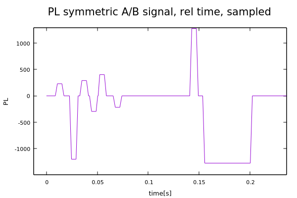
t2plot -t "PL symmetric A/B signal from flow start, zoom" -o 1:2 -sx 0:0.22 -ws 600,400 ~/results/film_flows_nps_srt_smpl.txt
This signal can be fed into any signal processing algorithm. Just read the sample in the sample file:
cat ~/results/film_flows_nps_srt_smpl.txt
0.000000        0
0.002500        0
0.005000        0
0.007500        0
0.010000        0
0.012500        231
0.015000        231
0.017500        0
0.020000        0
0.022500        0
0.025000        -1200
0.027500        -1200
0.030000        0
0.032500        0
0.035000        291
0.037500        291
0.040000        0
0.042500        0
0.045000        -294
0.047500        -294
0.050000        0
...
So you see, gnuplot does not show the PL 0 in the chosen plot mode, but they are there in the sampled file.
BPB measure
For AI researchers who are just interested in acquiring the best feature for their Neural Net without regarding the time dependence, the so called Bytes-Per-Burst (BPB) measure can be approximated by the sum(PL) pulse signal.
The nFrstPkts plugin has a NFRST_PLAVE configuration flag which can be used for this purpose:
grep -Fw NFRST_PLAVE $T2PLHOME/nFrstPkts/src/nFrstPkts.h
#define NFRST_PLAVE 1 // 1: Packet Length Average; 0: Sum(PL) (BPP); if (NFRST_MINIATS|NFRST_MINIATU) > 0Let us switch it to 0 with t2conf:
t2conf nFrstPkts -D NFRST_PLAVE=0
t2build nFrstPkts
t2 -r ~/data/film.pcap -w ~/results
fpsGplt -f 13 -i -s ~/results/film_flows.txtGenerating '/home/wurst/results/film_flows_nps.txt'... OK Generating '/home/wurst/results/film_flows_nps_srt.txt'... OK
t2plot -t "PL symmetric A/B signal from flow start, rel time, zoom" -o 1:2 -sx 0.015:0.22 -pl -ws 600,400 ~/results/film_flows_nps_srt.txt
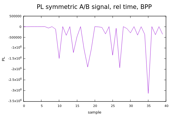
Choose a higher NFRST_MINIATU according to your detail requirements of the classification process, remove the time info and you have the Bytes-Per-Burst (BPB) measure.
fpsGplt -f 13 -i -t -s ~/results/film_flows.txtGenerating '/home/wurst/results/film_flows_nps.txt'... OK Generating '/home/wurst/results/film_flows_nps_srt.txt'... OK
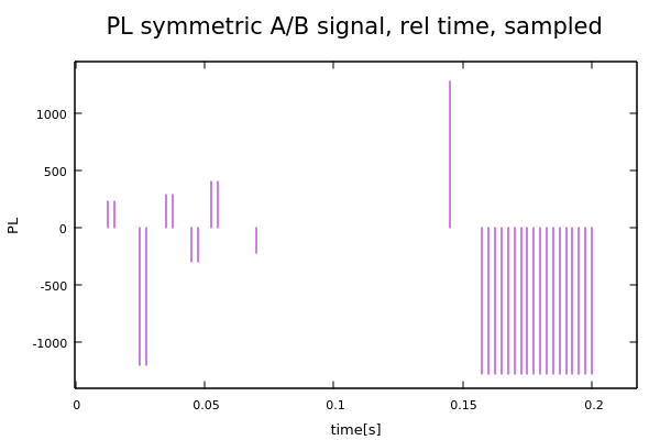
t2plot -t "PL symmetric A/B signal, flowInd 13, rel time" -o 1:2 -pl -ws 600,400 ~/results/film_flows_nps_srt.txt
If you need it non inverted, omit the -i option.
Now what? What can you do with it now? That is discussed in our next AI tutorial Classification of encrypted video streams.
Conclusion
Do not forget to reset all constants if you want to follow other tutorials:
t2conf nFrstPkts -D NFRST_IAT=1 -D NFRST_BCORR=0 -D NFRST_MINIATU=0
t2build nFrstPkts